My Soundtrack

I’ve always felt that music transcends words to construct a boundless language of its own, and it’s precisely because of this that I struggle to articulate what I love about a song. I tend to react quite instinctively and impulsively to a melody, and I’ve usually decided within the first listen whether or not it will be a favorite of mine. My favorite songs can bring me to emotional extremes, but I can’t always explain why. Is it the beat, or a chord progression, or the words or a random combination of each? Or is it something more intangible?

As my relationship with music is extremely special to me, I could not think of a better segue into the world of predictive modeling than attempting to answer these questions. I am excited to follow my curiosity for culture and data into future projects like this one that can lead me to discover more about human interaction with the world around us.

I went through several revisions of how to add a predictive aspect to this project, given that I did not have access to my own streaming data or a quantifiable way to determine which songs were my favorites. I settled on using a curated playlist of mine that accurately represents my taste in music to compare audio features against those of my entire saved Spotify library.

Import Libraries

I started by importing all the libraries I would use throughout the course of the project. I also set certain variables that I know I would be using repeatedly. In order to prevent my Client ID and Client Secret (created by starting a Spotify Web App) for being on display, I set environment variables and passed them here by importing the module environ from the library os.

Import Libraries

   import spotipy
   import pandas as pd
   import time
   import datetime as dt
   import numpy as np
   import seaborn as sns
   import matplotlib.pyplot as plt
   import itertools as it
   from os import environ
   from spotipy.oauth2 import SpotifyClientCredentials
   from scipy.stats import ttest_ind

Set Variables

   client_id = environ['SPOTIPY_CLIENT_ID']
   secret = environ['SPOTIPY_CLIENT_SECRET']
   redirect_uri = environ['SPOTIPY_REDIRECT_URI']
   user_id = '12179890696'
   scope = 'user-library-read'

Pass in Chosen Playlist IDs

   train_playlist = '4lexbQSIJBWtJGQS3GQkUC'
   test_playlist1 = '37i9dQZF1DWWBHeXOYZf74'
   test_playlist2 = '37i9dQZEVXbrG9oAilGQPt'
   test_playlist3 = '37i9dQZEVXcEQDzu8ByiUH'

Spotify Web API

I was able to obtain data for a given playlist using Spotify’s Client Credential Flow, but since I was reading my user library data as well, I also needed to use the Authorization Code Flow, which grants access to user data based on the user’s permission. Read more on Spotify’s Authorization Guide. Below is the process I followed to set up the Authorization code flow:

sp_auth = spotipy.Spotify (                                                                                                                                                   
    auth_manager=SpotifyOAuth (
        client_id=client_id,                                              
        client_secret=secret,                                      
        redirect_uri=redirect_uri,
        scope=scope
    )
)

Data Collection

When I thought about what songs I wanted to use to train the model to predict songs that I would love, I immediately settled on the Spotify playlist that I have been adding to for years, containing the songs that evade categorization in my mind, the ones that make me feel the most like myself when I listen to them. I have no real logic for adding a song to this playlist, aptly titled “me”, I just know when I hear it.

I pulled back the metadata and audio features for the songs in this playlist as well as for my entire saved library. In order to do this, I wrote four separate functions:

Get a list of track IDs in a playlist (no authorization required)

   def getTrackIDs(user, playlist_id):
       ids = []
       playlist = sp.user_playlist(user, playlist_id)
       for item in playlist['tracks']['items']:
           track = item['track']
           ids.append(track['id'])
       return ids

Get a list of track IDs from a user’s library (authorization required)

   def libraryTrackIDs():
       results = sp_auth.current_user_saved_tracks()
       tracks = results['items']
       while results['next']:
           results = sp_auth.next(results)
           tracks.extend(results['items'])
       library_ids = []
       for item in tracks:
           track = item['track']
           library_ids.append(track['id'])
       return library_ids

Break the list of IDs into sublists of 50 IDs (bypasses 50 track limit for the Get Several Tracks endpoint

   def divide_chunks(ids, n):
       id_chunks = []
       for i in range(0, len(ids), n):
           chunk = ids[i:i + n]
           id_chunks.append(chunk)
       return id_chunks

Return audio features for a given list of IDs

   def getTrackFeatures(ids):
       meta = sp.tracks(ids)
       features = sp.audio_features(ids)
       tracks = []
       for i in range(len(meta['tracks'])):  
           track = meta['tracks'][i]
           # metadata
           name = track['name']
           album = track['album']['name']
           artist = track['album']['artists'][0]['name']
           release_date = track['album']['release_date']
           length = track['duration_ms']
           popularity = track['popularity']
           explicit = track['explicit']

           # audio features
           key = features[i]['key']
           mode = features[i]['mode']
           time_signature = features[i]['time_signature']
           acousticness = features[i]['acousticness']
           danceability = features[i]['danceability']
           energy = features[i]['energy']
           instrumentalness = features[i]['instrumentalness']
           liveness = features[i]['liveness']
           loudness = features[i]['loudness']
           speechiness = features[i]['speechiness']
           tempo = features[i]['tempo']
           valence = features[i]['valence']

           tracks.append((
               name, album, artist, release_date, length, 
               popularity, explicit, key, mode, time_signature,
               acousticness, danceability, energy, instrumentalness,
               liveness, loudness, speechiness, tempo, valence
           ))
       return tracks

Once these functions were written, the variables I defined earlier could be passed in as arguments to retrieve the data. Below is an example of the function in use, passing in my “favorites” playlist ID (train_playlist).

ids = getTrackIDs(user_id, train_playlist)
id_chunks = divide_chunks(ids, 50)

favorite_tracks = []
for id_chunk in id_chunks:
    for track in getTrackFeatures(id_chunk):
        favorite_tracks.append(track)

Once I completed the audio feature retrieval for every track, I concatenated the two dataframes into a larger dataset and removed duplicates. I created a column titled “favorite”, and placed 1’s next to all of the tracks in my favorites playlist and 0’s next to the rest. The total dataset consisted of close to 2,000 observations, with 90 of them being marked as “favorite”. Below is a sample of the data:

I repeated the process for the “test” data by concatenating the audio features for three separate playlists (Release Radar, POLLEN, Discover Weekly) into a dataset that I would later run my trained model on.

Data Exploration

Once I had the data in a tidy format, I was able to inspect it more closely. There are 12 audio features available in Spotify’s Get Audio Features endpoint. The ones bolded below are within a Spotify-scored scale of 0.0 – 1.0.

Key
Mode
Time Signature
Acousticness
Danceability
Energy
Instrumentalness
Liveness
Loudness
Speechiness
Tempo
Valence

I first compared the means of two subsets (favorite and non-favorite tracks) of my dataframe using an independent sample t-test, and found there to be a significant difference in means (at the 0.05 alpha level) for mode, danceability, and speechiness, indicating that these three features could be strong signals for identifying a favorite track.

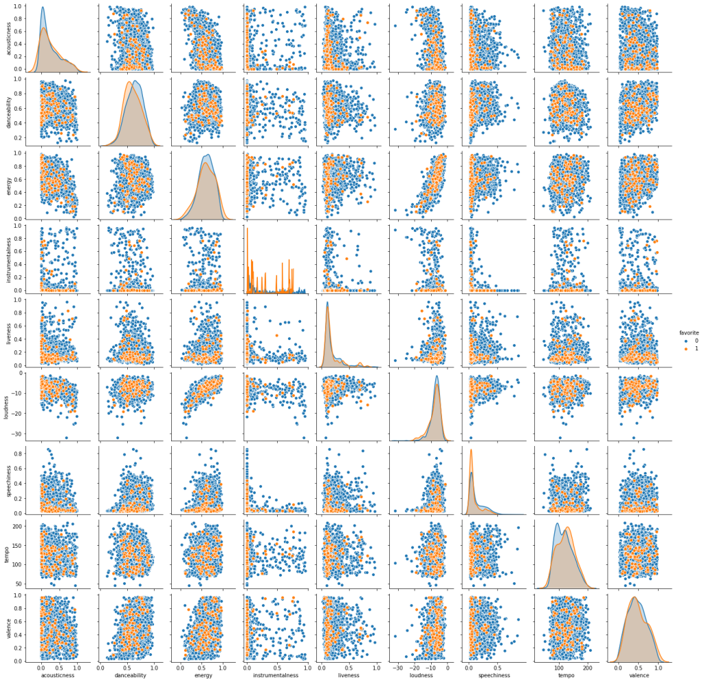
From the scatterplot grid (built using the pairplot function from the python library Seaborn) of all the continuous variable audio features below, it can be seen that my favorite tracks are more likely to be higher in tempo and lower in danceability score than the rest of my saved tracks.

I also inspected the correlation relationship (using the heatmap function from Seaborn) between each feature to see if one feature held influence on another within this data set.

I found that loudness and energy show a strong positive correlation, as does speechiness and explicit. Acousticness has a fairly strongly negative correlation with both energy and loudness.

Model Selection & Revision

I decided to test out two different classification algorithms to determine which yielded the highest accuracy rate: K-Nearest Neighbors and Random Forest.

K-Nearest Neighbors

K-Nearest Neighbors is a supervised machine learning method that classifies data based on the points that are most similar to it. It calculates the distance between the test data point and the predetermined k nearest data points, and classifies the test point based on what class the majority of the neighboring data points fall into.

I first normalized the data as is suggested for a distance-based algorithm.

audio_features_normalized = (audio_features - audio_features.mean()) / audio_features.std()

I then divided the data into a 75% training and 25% testing split.

audio_features_train, audio_features_test, target_train, target_test = train_test_split (audio_features_normalized, target, test_size = 0.25)

I then determined the optimal k by running the model through a range of k values (1-50) and calculating the error rate at each value to determine the k value at which the error rate was the lowest.

neighbors = list(range(1, 50, 2))
cv_scores = []

for k in neighbors:
    knn = KNeighborsClassifier(n_neighbors=k)
    scores = cross_val_score(knn, audio_features_train, target_train, cv=10, scoring='accuracy')
    cv_scores.append(scores.mean())

mse = [1 - x for x in cv_scores]

optimal_k = neighbors[mse.index(min(mse))]
print("The optimal number of neighbors is {}".format(optimal_k))

# plot misclassification error vs k
plt.plot(neighbors, mse)
plt.xlabel("Number of Neighbors K")
plt.ylabel("Misclassification Error")
plt.show()

Finally I ran the model with the optimal k neighbors and predicted the probabilities for the classification (non-favorite and favorite) of each data point in the audio_features_test set. This model scored 96%.

knneighbors = KNeighborsClassifier(n_neighbors=optimal_k, weights='distance')
knneighbors.fit(audio_features_train, target_train)
knneighbors.predict_proba(audio_features_test)

Re-running the model with cross validation achieved a 95% score.

This model predicted that it was 0% probable that I would place any of the songs in the test data in my favorites playlist. This is likely due to the low k-value and the small ratio of “favorite” songs as compared to “non-favorite” songs; the 7 neighboring points surrounding the test data point were likely all non-favorite tracks, resulting in a probability of 0 for a classification of “favorite”.

Random Forest

Random Forest models are also supervised learning algorithms, consisting of several (in this case, 100) random decision trees that merge together to create a more stable prediction.

To begin, I viewed the feature importances of all the audio features to see if there were any I could leave out without it affecting the model. Because I am using a Stratified K-Fold Cross Validation method to evaluate the model performance, I did not feel it was necessary to use a train/test split in this case.

#Features
features = alltracks_df[['key','mode','time_signature','acousticness','danceability','energy','instrumentalness','liveness','loudness','speechiness','tempo','valence']]

#Target
target = alltracks_df['favorite']

#Model
rf = RandomForestClassifier(n_estimators=100)

#Feature Importance
feature_imp = pd.Series(rf.feature_importances_,index=features.columns).sort_values(ascending=False)

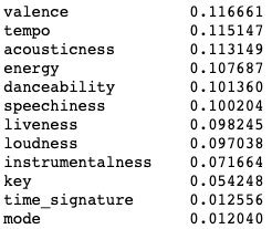
I then proceeded to choose 3 subsets of the data based on my own estimation of most influential features, feature importance as stated by the model, weak correlation, and statistically significant differences between favorite and non-favorite populations.

Subset 1: My Most Influential Features

In this subset I chose the features that I believe to be the most influential in my music taste: Valence, Energy, and Key. Valence and Energy both had high feature importances, whereas key had a very low feature importance in this combination. The cross validation score for this model was 94.9%.

#Features 
audio_features1 = features[['valence','energy','key']]

#Model
rf.fit(audio_features1, target)

#Feature Importance
print(audio_features1.columns)
rf.feature_importances_

#Cross Validation
results1_rf = cross_val_score(rf, audio_features1, target, cv=RepeatedStratifiedKFold(n_splits=5, n_repeats=10))
results1_rf.mean()

Subset 2: Features with Significantly Different Means

In this subset I chose the features that had significantly different means across the favorite and non-favorite groups (taken from the independent sample t-test conducted earlier). These features are Mode, Danceability, and Speechiness. Mode had a very low feature importance, and the other two had very high importances, with speechiness being the highest. The cross validation score for this model was 94.6%.

#Features 
audio_features2 = features[['mode','danceability','speechiness']]

#Model
rf.fit(audio_features2, target)

#Feature Importance
print(audio_features2.columns)
rf.feature_importances_

#Cross Validation
results2_rf = cross_val_score(rf, audio_features2, target, cv=RepeatedStratifiedKFold(n_splits=5, n_repeats=10))
results2_rf.mean()

Subset 3: Most Important Features

In the final subset, I chose to include all of the features with the highest importance from the previous models: Danceability, Speechiness, Valence, Energy, Loudness, and Tempo. The cross validation score for this model was 95.1%.

#Features 
audio_features2 = features[['mode','danceability','speechiness']]

#Model
rf.fit(audio_features2, target)

#Feature Importance
print(audio_features2.columns)
rf.feature_importances_

#Cross Validation
results2_rf = cross_val_score(rf, audio_features2, target, cv=RepeatedStratifiedKFold(n_splits=5, n_repeats=10))
results2_rf.mean()

Final Prediction

I chose to use the random forest model for my final prediction because it protects against overfitting, which was a concern of mine as all of my favorite tracks have quite a large variance within each feature. It also allowed me to inspect feature importance, which helped me get a better sense of which features were contributing the most to song classification within my dataset; I was able to test different combinations of features to optimize the model.

Of the three subsets, subset 3 yielded the best results, so I used that to fit the final model.

#Features
features_rf = audio_features3

#Final Model
rf_final = rf.fit(features_rf, target)

#Features for Untrained Data
features_test_rf = testtracks_df[['danceability','speechiness','valence','energy','loudness','tempo']]

#Final Predictions
predictions_rf = rf.predict(features_test_rf)

#Loading Predictions into Test Dataframe
testtracks_df['rf_favorite'] = predictions_rf

#Loading % Likelihood of "favorite" Classification
rf_likelihood = rf_final.predict_proba(features_test_rf)
testtracks_df['rf_likelihood'] = rf_likelihood[:,1]

Results

The model correctly identified two tracks that I had already added to my favorites playlist: “Dead Man Walking” by Brent Faiyaz and “Good Days” by SZA. I also really loved “Take Care In Your Dreaming” (30%) and “Back on the Fence” (19%). There were a few others sprinkled throughout the results that I liked, but would not make the cut for my favorites playlist.

Going Further

In seeing that the probabilities for classification into my favorites playlist was quite low across the board I think there are two factors that are contributing to this:

My “favorite” tracks are too varied across all the features, leading to highly specific data points which possibly led to overfitting.
There are not enough data points in the “favorite” subset to create a large enough picture of my ideal song.

In my next steps, I would like to create a more robust set of “favorite” songs, perhaps using the personalized Spotify-curated playlist Your Top Songs 2020 that is based on a quantifiable metric rather than self-curation. I would also consider widening the parameters of what makes a “favorite”, so I can get a more varied likelihood score. It would also be really interesting to compare the results of the model trained on that playlist with those of the previous years’ Your Top Songs playlists, to see if and how my taste has changed over the years.

Next, I would also like to create a song “archetype” from my favorite songs, using K-means clustering to group similar tracks and create my own personal “genres”. This would allow me to run this same classification model on each “genre” separately, and would therefore eliminate the overfitting issue.

Exploring my own music taste through the lens of data was an awesome learning experience. However, I will be the first to admit that there are just some things that get me excited about a song that can’t be captured, such as a charming chord progression, a frenzied crescendo of a guitar solo, a mysteriously echo-ey synth beat, or an emotion-laden voice.